Mathematics Developmental Continuum

Success depends on students finding the median of an odd-numbered set of numerical data and appreciating qualitatively how the median is affected by the inclusion of new data.
This is the second ‘central measure’ that students will experience; they have already used ‘mode’ (Level 3.25) and they are yet to meet ‘mean’ (Level 4.0).
At this level, they find the median from an even-numbered set by estimating or intuitively identifying the average of the two middle values, or simply saying it is between them. Later, they will find the median through the (weighted) mean of the middle two data values. The distinctions that are made at later levels between discrete numerical data (like shoe sizes) where no intermediate values are possible and continuous numerical data (like height) are not made at this level.
For more information, related indicators are:
Students first become familiar with categorical data (such as football teams, favourite pets and colours) and understand that the most popular team, colour or pet can be found by voting. The category with the most votes is the ‘mode’. The mode is the only statistic suitable for categorical data.
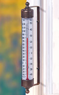
The next step is to apply the concept of mode to numerical data. For example, if we read a thermometer outside the classroom every day at 1:00 p.m. and record the temperatures for a month then we might find the mode 1 pm temperature for February is 30 degrees and the mode for May is 22 degrees. These modes are the most common temperatures for those months and might be used for month-to-month comparisons.
While it is possible to use the mode for describing both categorical and numerical data, the median is useful only for data that can be ordered from smallest to largest (usually numerical).
If the 1 pm temperatures for every day of May were listed in order from the minimum to the maximum, the median is then the middle score. Sometimes the median is the same as the mode, but not always. For example, if the 1pm temperatures every day for a week were 22°, 22°, 22°, 20°, 26°, 25°, 24° then the mode and the median are both 22°. If instead the 20° day had a temperature of 29°, then the mode remains 22°, whilst the median is 24°.
Both the median and the mean are useful for summarising numerical data. The advantage of the median is that, as it is based on the simple process of ordering, it is easier to calculate than the mean. The disadvantage of the median is that it is not reflective of all the data set in the way that the mean is. The mean also has stronger mathematical properties, so it is used in advanced statistics.
These activities are based around a set of 15 data cards which students arrange in various ways as they focus on the different data provided on the cards - Data cards small (PDF - 351Kb).
Larger versions of these cards are also provided for teacher’s use - Data cards large (PDF - 827Kb).
Students can use class data for later work. Each of the activities proceeds in four steps:
Step 1: Recognise variation in the data set by noting
individual values and looking at the range
Step 2: Group
the data by looking for patterns, calculating frequencies, column graphs etc
Step
3: Represent the data with mode, median and range
Step 4:
Explore properties of the mode, median and range.
Activity 1: T-shirts reviews students’ knowledge of
the mode for categorical data, using the four steps above.
Activity
2: Heights introduces the concept of the median, which applies to
numerical data, using the four steps above.
Activity 3: Pets,
shoe sizes and travel times establishes the work on median, mode and
range in three different contexts, each using the four steps above.
Activity
4: Comparing groups splits the data set into 2 groups and
students describe the differences between them, using mode, median and range.
At this level, students do not deal with relationships between two numerical
variables (e.g. shoe size and height).
Ask students questions about the data cards (see the suggestions below) focussing on the categorical variable of T-shirt design to review their knowledge of grouping, mode etc.
Step 1: Recognise variation in the data set, by noting individual values and looking at the range.
Students should group their cards according to the T-shirt design to answer the questions. Note that as this variable does not have any inherent order, the students may arrange their groups of cards in many different (acceptable) ways. This is in contrast to the numerical data such as number of pets in later activities.
Step 2 : Group the data by looking for patterns, calculating frequencies, column graphs etc
These questions focus on one category at a time and then compare categories:
Arranging the cards in rows or columns based on T-shirt design will lead to a pictograph (using cards as objects on the graph) and then to a column graph similar to that shown below.
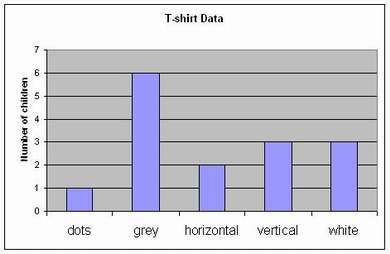
| T-shirt | Number of children |
| dots |
1
|
| grey |
6
|
| horiz. stripes |
2
|
| vertical stripes |
3
|
| white |
3
|
Step 3: Represent the data with mode (no median yet)
This is called the ‘mode’: it occurs more often than any other T-shirt.
If
you owned a T-shirt shop, you would probably keep more grey T-shirts than any
other colour.
Step 4: Explore properties of the mode
A new student, Tara, is about to join the other 15 students already on the data cards.
Five new students are put onto the data cards.
This activity introduces the concept of the median as the middle value, seen when the data cards are arranged in order. This is numerical data, so whilst the cards can be grouped as in Activity 1 above, there is an inherent order between the groups. Students should be able to see the different heights of the children on the cards, as well as using the data on the cards.
Step 1: Recognise variation in the data set by noting individual values and looking at the range
Students ask and answer questions focusing on the individual values. For example:
Step 2: Group the data by looking for patterns, calculating frequencies, column graphs etc
Students look at the data in groups, focusing on one category at a time.
Summarise these investigations with tables and charts.
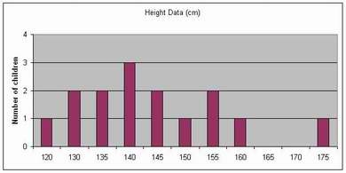
| Height | Number of children |
| 120 |
1
|
| 130 |
2
|
| 135 |
2
|
| 140 |
3
|
| 145 |
2
|
| 150 |
1
|
| 155 |
2
|
| 160 |
1
|
| 165 |
0
|
| 170 |
0
|
| 175 |
1
|
Step 3: Represent the data with mode, median and range
Arrange the data cards in order of height.
Here is one possible arrangement of the cards based on heights, from shortest to tallest. Note that students of the same height can be rearranged. Once the cards are ordered, a new statistic (the median) can be introduced. It is another ‘central measure’ like the mode. Note that the mode is 140 even if the cards are rearranged and Sue is the middle card instead of Dave.
|
120 |
130 |
130 |
135 |
135 |
140 |
140 |
140 |
145 |
145 |
150 |
155 |
155 |
160 |
175 |
|
Amy |
Mark |
Fay |
Ian |
Pete |
Sue |
Cath |
Dave |
Bill |
Gail |
Tom |
Nora |
Jeff |
Luke |
Ruth |
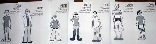
The image below shows the middle seven cards from the above arrangement. There is a strong visual image of the median height being the height of the middle child.
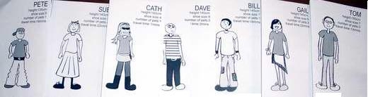
Report the 3 statistics: range, mode and median.
The median height is 140 cm; the median is the middle value when the heights are arranged in order. Note: in this example, the median is the same as the mode, both 140 cm. This is not always the case, they can be different numbers (see Illustration 2).
Step 4: Explore the properties of the mode, median and range
To explore how the median, mode and range work, set students the task of designing cards for 2 new students Tara and Wong, so that:
Students can arrange themselves in order of height to find the median height for their own group.
Activity 2 above, illustrated with heights, is repeated for three different variables:
For each variable, follow the four steps as illustrated in Activity 2, gradually reducing the support offered for finding the median.
Step 1: Recognise variation in the data set, by noting
individual values and looking at the range
Step 2: Group
the data, by looking for patterns, calculating frequencies, column graphs etc
Step
3: Represent the data with mode, median and range
Step 4:
Explore the properties of the mode, median and range.
When the cards are put in order of these other variables, the median is not obvious from the visual arrangement, but it is still the middle card.
Number of pets
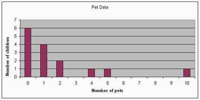
|
Number of pets |
Number of children |
|
0 |
6 |
|
1 |
4 |
|
2 |
2 |
|
3 |
0 |
|
4 |
1 |
|
5 |
1 |
|
6 |
0 |
|
7 |
0 |
|
8 |
0 |
|
9 |
0 |
|
10 |
1 |
|
0 |
0 |
0 |
0 |
0 |
0 |
1 |
1 |
1 |
1 |
2 |
2 |
4 |
5 |
10 |
|
Amy |
Mark |
Ian |
Dave |
Tom |
Jeff |
Pete |
Cath |
Bill |
Luke |
Gail |
Nora |
Sue |
Ruth |
Fay |
Note that the mode and the median remain the same (0 and 1 respectively) even if the cards of people with the same number of pets are rearranged (e.g. if Pete and Cath are swapped).
The image below shows the middle seven cards from the above arrangement. Note the contrast with the image of heights; the attribute of height is no longer the basis for this activity.
For Step 4, ask questions such as:
Shoe Size
Here is one correct ordering of cards from smallest shoe to largest. The median shoe size is 6.
|
3 |
4 |
4 |
5 |
5 |
5 |
5 |
6 |
7 |
7 |
7 |
7 |
8 |
9 |
11 |
|
Mark |
Amy |
Cath |
Fay |
Ian |
Pete |
Sue |
Gail |
Bill |
Tom |
Nora |
Ruth |
Dave |
Luke |
Jeff |
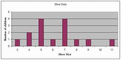
|
Shoe Size |
Number of children |
|
3 |
1 |
|
4 |
2 |
|
5 |
4 |
|
6 |
1 |
|
7 |
4 |
|
8 |
1 |
|
9 |
1 |
|
10 |
0 |
|
11 |
1 |
Students can divide the data cards into groups, such as boys and girls. They can compare height, shoe size, number of pets and travel time for these two gender groups. They can also compare the categorical data (T-shirt colour, shoe colour, etc).
In each case, students will:
*Note: Finding the median for the 8 boys presents a new problem. Whereas there is always a middle person in the set of 7 girls, there is never a middle person in the set of 8 boys. To overcome this, students can either say the median is 'between 140 cm and 145 cm' for height, or they can take the number halfway between. Many students will know this is 142.5 cm, which is the average/mean of the two middle values.
The following resource contains sections that may be useful when designing learning experiences:
Digilearn object *
Rice
crisp machine – students check whether a machine is packing most bags with
an acceptable number of rice crisps (20–35 rice crisps per packet). Students
take a sample of 100 packets and make a boxplot to analyse the results.
Students sort the sample data into four equal groups. Students identify the
range, median, first and third quartile values.
(https://www.eduweb.vic.gov.au/dlr/_layouts/dlr/Details.aspx?ID=4431)
* Note that Digilearn is a secure site; DEECD login required.