Short-Run Variation and Long-Run Stability: 5.0
Supporting materials
Indicator of Progress

Students know random processes exhibit short-run variation and they also exhibit long-run stability. They understand that if they roll a fair die 10 times then the proportion of sixes is hard to predict, but if they roll it 10000 times, the relative frequency is highly likely to be very close to 1/6, the theoretical probability. In this way, the relative frequency gives the experimental (empirical) probability, which approximates the theoretical probability.
Prior to this, some students focus on the unpredictability of individual events, and have difficulty in reconciling this with the predictability of the long-run relative frequency of an outcome. Other students overgeneralise the predictability of the long-run relative frequency and so over-estimate the predictability of individual events.
Illustration 1: Diagnostic task
Ideas of short-run variability and long-run stability develop slowly. From experiences playing games with dice, many quite young students will know that if a die is rolled six times they would not expect to see each possible outcome once {1, 2, 3, 4, 5, 6}. Students will understand that there is variation in results obtained from rolling a die, but it is likely that they have only considered numbers of outcomes rather than consider the long-run relative frequency of obtaining each outcome that is essential at this level.
The question below asks students to compare probabilities. In senior mathematics, they will learn to calculate these probabilities, but at this level, the intention is that they begin to build up intuition about the extent of variation, and learn to focus on relative frequency. With modern technology providing simulations, it is possible to develop more intuition than is possible with hands-on experiments only.
A fair coin is tossed. Which outcome is more likely, or are they equally likely? Give your reasons. (Correct answers italicised)
(a) Getting exactly 5 heads when you toss a coin 10 times OR getting exactly 500 heads when you toss a coin 1000 times?
(b) Getting 4, 5 or 6 heads when you toss a coin 10 times OR getting 499, 500 or 501 heads when you toss a coin 1000 times?
(c) Getting 4, 5 or 6 heads when you toss a coin 10 times OR getting between 400 and 600 heads when you toss a coin 1000 times?
Part (a) will be answered incorrectly by students who over-estimate the predictability of individual events and those with a shallow understanding of the short-run variability and long-run predictability.
Parts (b) and (c) are designed to identify those students who appreciate the importance of the relative frequency, not just frequency of outcomes.
Students may answer part (b) incorrectly if they know that there is long-run predictability (about a half will be heads) but think about this in absolute terms, rather than relative frequency. It is much more likely to be within 1 of half when tossing 10 times than to be within 1 of a half when tossing 1000 times.
Part (c) also tests whether students are thinking about relative frequency. Correct answers should mention that the relative frequencies are the same (4 - 6 heads or 400-600 heads) but the increasing number of tosses means that that the number of heads is more likely to be about a half when there are more tosses.
Teaching Strategies
Students will already be familiar with ideas of unpredictability of random processes and possibly also with ideas of long-run predictability, but these are subtle ideas which need development and discussion over some time.
The activities below are sequential, and employ the principles that teaching about probability and random processes should be based in practical experiences and that technology can be used to extend classroom experiences from the hands-on base.
Activity 1: Small number of trials exhibit great variation is an awareness raising activity, providing hands-on experience, and moving students towards the conceptual change of considering rolling a die 12 times as one experiment (and not 12 experiments).
Activity 2: Exploration of 60 trials makes the transition from hands-on experience to using the random number generator in a spreadsheet to explore the variation in samples of 60 rolls of a die, with results presented numerically and graphically.
Activity 3: Exploring long-run relative frequency, experimental and theoretical probability extends the exploration using technology to experiments consisting of 6000 trials, conducted multiple times. Students can directly compare the variability of experimental probabilities from short-run and long-run experiments.
These activities assume familiarity with basic ideas of probability such as understanding why the probability of getting a 3 on a roll of a fair die is 1/6.
A spreadsheet is used here to enable rapid execution of a large number of trials with high standards of randomness, and rapid graphical display of the results. Without technology, data collection is limited, but if students work together, a large data set can be collected fairly quickly. Do not assume that all students will appreciate the relevance of the the computer graphics, which will certainly need careful attention.
Activity 1: Small numbers of trials exhibit great variation
The main purpose of this activity is to give students experiences with the unpredictability of rolling dice and considering the likelihood of obtaining a given outcome. For students who may not have played many board games this is an important first stage. Students develop the notion that there is variation in the frequency of particular outcomes for small numbers of trials. It also establishes the idea that a set of twelve rolls of the dice is one experiment.
Predict. Have students predict how many 3s they would get if they rolled a die twelve times and explain their reason. Also ask them to predict the maximum number of 3s that might be obtained as well as the minimum number.
Experiment. Have students roll a die twelve times (or roll twelve dice once) and record the number of times each outcome occurs.
Discuss. Discuss the variation in the results for different students, noting that outcomes do not usually occur the same number of times, and that students will get different results. Compare number of 3s with predictions.
Calculate. Each student should work out the relative frequency of each outcome {1, 2, 3, 4, 5, 6} based on their own trials and record these as their own experimental probabilities.
Discuss. Conduct a class discussion of the variation in the values of the experimental probabilities obtained by different students.
Activity 2: Exploration of 60 trials
This activity extends the previous activity by using a simulation of rolling a die sixty times, which enables students to explore the variation in the relative frequencies (experimental probabilities) with a larger number of trials. Students interpret both tabulated and graphical data to determine the variation in results for this situation.
Step 1: 60 trials with a die
Ask students to predict how many ones, twos, threes, fours, fives and sixes they would they get if a die was tossed 60 times. Students should predict around 10 as this is the expected value (i.e. the average). Get pairs of students to roll a die sixty times and record the number of times each outcome appears. Students should write down the frequency of each outcome and convert to its relative frequency (i.e. divide by 60). Discuss the variation in the results. For example, did anyone get exactly ten of each outcome? Did anyone not have any threes, etc.? What was the highest frequency for an outcome?
Link relative frequency and experimental probability. Note that students need to consider each set of 60 trials as one experiment, not as 60 experiments.
Step 2: 60 trials with a random generator, adding an automatic graphical display
Now get students to use a random number generator in a spreadsheet to simulate 60 rolls of a die.
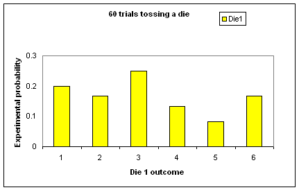
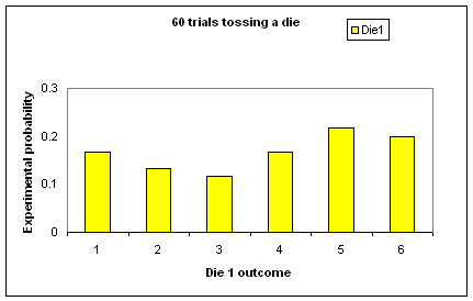
Use the 60 trials page of the attached spreadsheet (Excel - 802Kb) (or see instructions for constructing your own spreadsheet). Each time the spreadsheet file opens, 60 rolls of a die are automatically generated. Get students to write down the relative frequencies (experimental probabilities) and use the summary table and graph to describe the situation for one group of 60 rolls. Two graphs for 60 rolls are shown below.
Discuss the range of results in the class, with similar questions as before. Also ask: What are the biggest differences in experimental probabilities for a sample of 60? The vertical axis of the spreadsheet graph only goes up to 0.3 - is this high enough? Ask students to explain how the experimental probabilities are calculated, ensuring the link to relative frequency is clear.
 |
 |
Step 3: Exploring the variations in experimental probabilities found from 60 trials
Now have students perform many trials using the spreadsheet and focus on the variation in different groups of 60 trials. To generate many simulations of rolling a die 60 times, press CTRL = . Have students describe the variation in the results overall for situations where a die is rolled 60 times. In this case they are looking at the notion of variation overall, rather than specific numbers of outcomes for a single set of 60 trials. A class discussion will highlight that the experimental probabilities are not constant for 60 trials, but students can predict a range that they might expect these values to lie within. Comment that 60 trials still exhibit considerable variation in results; very likely more than was expected.
Activity 3: Exploring long-run relative frequency, experimental and theoretical probability
In this activity students use the random generator in the spreadsheet (Excel - 802Kb) to produce many results of many trials quickly to explore long term relative frequency and the experimental probability.
Students will observe how the variation in results for each experiment is larger for experiments with a smaller number of trials. They will also observe that when the number of trials is very large, the value of the experimental probability (long-run relative frequency) is often very close to the theoretical probability.
Step 1: 600 trials repeatedly, and then 6000 trials repeatedly
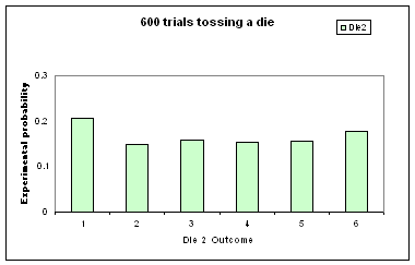
Clicking onto the second sheet of the spreadsheet generates results for rolling the die 600 times. Typing CTRL = generates results for rolling another 600 times.
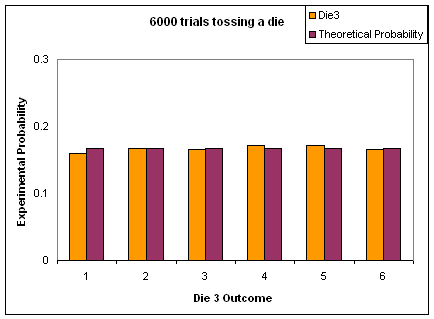
Clicking onto the third sheet of the spreadsheet generates results for rolling the die 6000 times. Typing CTRL = generates results for rolling another 6000 times.
Students start by considering 600 rolls of a die and then consider 6000 (see below for sample graphs).
Students should describe the results in each case and note features of the graphs. For example, for the 600 trials, students should observe that the relative frequencies are nearly always between about 0.1 and 0.2 and there is less variation than was observed for the 60 trials. What is important here is to get students to consider many graphs and comment on the overall trend in the value of the experimental probabilities.
Having the theoretical probability on the graph for 6000 trials shows how the relative frequency for each outcome has a value close to the theoretical probability. There is much less variation. Whilst there is short-run variation, there is long-run stability.
 |
 |
Step 2: Less variation when there are more trials
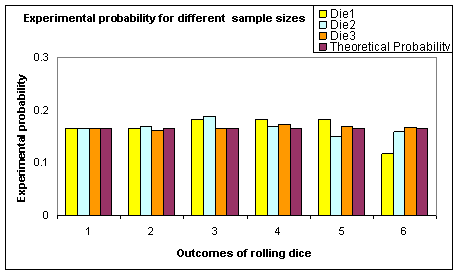
Students can now consider a graph showing simulations for 60, 600 and 6000 rolls of a die on one set of axes. This is the fourth sheet, called CompareTrialsTheoretical in the spreadsheet.
It is useful to let students observe the variability by running the random generator (CTRL =) many times. They can then discuss the variation in long-run relative frequencies for 6000 rolls of a die compared to 60 and 600 rolls of a die. Even for 6000 trials, there is still some variability in the relative frequencies and hence the experimental probabilities. This is evident in the amount of movement in the graph.
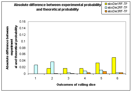
The second graph below shows the absolute difference between the long-run relative frequencies and the theoretical probability. It is a further graphical display to show that the experimental probability is close to the theoretical probability when the number of trials is large. This further reinforces the ideas of short-run variation and long-run stability.
 |
 |
Step 3: Variations
Further activities could include exploration of cases where outcomes are not equally likely. Teachers could set up a spreadsheet (click here for advice) where the probabilities of three outcomes are ½, ¼ and ¼, or combine some outcomes on this spreadsheet.
